2.5. Create a Water Quality Map
This guideline provides information about the Water Quality application of the Hydrology Thematic Exploitation Platform (HTEP). Simultaneously this document provides a hands-on tutorial showing you how to produce a water quality map of your area of interest using the application in combination with the various features of HTEP.
2.5.1. Water Quality Application: An Introduction
It is of essential importance to be able to monitor temporal and spatial dynamics of inland water quality in order to obtain improved understanding of aquatic ecosystems. Making use of remotely sensed earth observation (EO) data is an efficient and cost-effective method to assess a variety of physical and biological parameters in aquatic ecosystems over large areas. The thematic application Water Quality (WQ), developed by EOMAP, is able to map these aquatic ecosystems. Combining this application with the features of the Hydrology Thematic Exploitation Platform (HTEP) ensures EO data can be easily accessed, processed, reproduced and shared with the hydrology community. In this tutorial the functionalities and features of HTEP using EOMAPs WQ application are discovered. Chapter 2.5.1.1 discusses important information about the WQ application: the advantages of using EO data over conventional measurement methods and the currently available in- and outputs for the application. The introduction is followed by a hands-on tutorial in Chapter 2.5.2, showing you how to use this application in combination with HTEP.
2.5.1.1. About EOMAPs Water Quality App
EO satellite data for monitoring of water quality yields a wide variety of advantages compared to conventional in-situ measurements. The usage of EO data means low costs and low labour intensity, easy mapping of large areas and a high spatial resolution in contrary to conventional in-situ measurements. Furthermore near real-time monitoring is possible using satellites with high temporal resolution and physically inaccessible areas can be covered. Besides the accuracies are high, typically only 20-30% deviation from in-situ measurements.
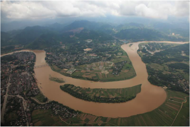
Figure 1: Red River, Vietnam
2.5.1.1.1. Water Quality Application Input
As input for the WQ application, there is EO data available of multiple satellite sensors, with varying spatial, temporal and spectral resolution. For the WQ application there is currently Sentinel-2 and Landsat-8 EO data available:
Sentinel-2 High Spatial, Weekly Temporal Resolution
The maximum spatial resolution of the output products of the WQ application is approximately 30 meters using Sentinel-2 data[1]. Sentinel-2 has a monthly revisit of approximately 5 times, meaning a weekly temporal resolution.
Landsat-8 High Spatial, Weekly Temporal Resolution
Landsat-8 has a maximal spatial resolution of about 30 meters, equal to Sentinel-2 data products. The temporal resolution of Landsat-8 is 16 days[1]. Therefore both Sentinel-2 and Landsat-8 data products are ideal for large scale monitoring of most relevant lake and river sizes. The spectral bands of Sentinel-2’s sensors range between 490 and 1375 nm and Landsat-8’s sensors range between 433 and 2300 nm[3] [4]. However, the output parameters of EOMAPs WQ app are based on backscattering of light between 400-850 nm, in the visible spectrum.
2.5.1.1.1.1. Influence of obstructions such as clouds on the results
Multiple considerations are needed to decide what data products are usable for the WQ app. As mentioned in the previous paragraph, output parameters of the WQ app are determined based on backscattering of light within the visible spectrum. Wavelengths in the visible spectrum cannot properly penetrate obstructions such as clouds and haze, meaning those kind of obstructions sometimes result in difficult measuring conditions. In addition, particular geometrical conditions between sun, target and sensor in combination with specific sea-state-conditions (wind speed, direction) can result in signal distorting mirroring effects, called sun glint, on the water surface. Other circumstances influencing the results include cloud shadows, shallow waters, disturbances by floating materials and mixed land-water pixels. Those pixels are flagged in the results, as will be discussed in Section 2.5.2.5. However, as clear as possible data images contribute to more reliable results. As such special care is required in terms of cloud coverage and sun glint. There are no guidelines for allowed cloud cover percentage, but a reduction in cloud coverage will improve the quality of the output products.
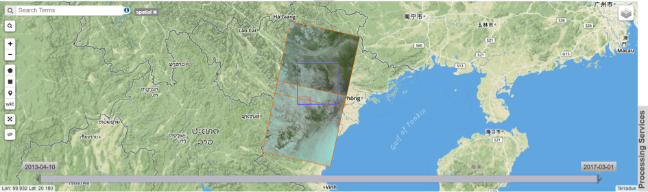
Figure 2: Landsat-8 Observations of Hoa Binh Reservoir, High Cloud Coverage
2.5.1.1.2. Water Quality Application Output
The output products the WQ app is able to generate are the following four main water quality parameters and an atmospheric correction:
- TSS Total Suspended Solids
The total suspended solid is the dry-weight of scattered particles in the water column. The influence of TSS on aquatic ecology is for example the negative effects on plants and animals due to a reduction of available light.
- CHL Chlorophyll
A pigment included in phytoplankton cells that serves as a proxy for algae in natural waters. The amount of chlorophyll is a measure for water quality, as it relates to algae biomass which can for instance result in decreased levels of dissolved oxygen.
- CDOM Colored Dissolved Organic Matter
CDOM absorbs light at the blue end of the visible spectrum, therefore being responsible for the water colour. Increasing CDOM, primarily caused by tannin due to decaying detritus, causes the water colour to go from blue, green to brown. The amount of CDOM importantly affects aqua systems: an overdose of CDOM may for instance result in a lack of available light for phytoplankton populations to grow, while phytoplankton is the basic of oceanic food chains and important for atmospheric oxygen.
- SWT Surface Water Temperature
SWT speaks for itself, as it means the WQ app is able to determine the temperature at the surface of a water body at the top skin, also known as the epilimnic temperature. Water surface temperature knowledge is important in aquatic ecosystems to better determine and predict for instance wind streams introduced by temperature differences.
- Atmospheric corrected product
Consists of satellite imagery which has been corrected for the effects of the atmosphere and scattering light from adjacent land and water surfaces. It provides reflectance data instead of scaled radiances or top-of-the atmosphere products and improves satellite imagery by minimizing effects of haze and atmospheric aerosols.
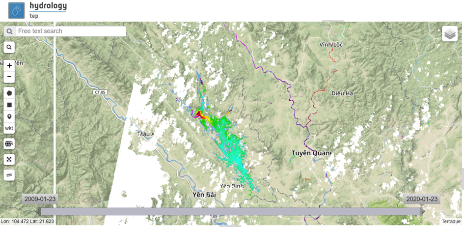
Figure 3: WQ App result on HTEP: TSS of Yen Binh Water Reservoir in the Red River basin
2.5.2. Tutorial: Producing a Water Quality Map of My Area of Interest
This chapter contains a hands-on tutorial how to work with EOMAPs WQ application on HTEP. The tutorial shows and explains step-by-step the different features of HTEP and the actions to be taken in order to create the Water Quality map of Figure 3. For this tutorial, the area of interest is the Yen Binh water reservoir in the Red River basin.
2.5.2.1. Accessing the Water Quality Thematic Application
- Enter the HTEP Community Portal and Sign in with your HTEP community user account. There is no preferred internet browser. However, for this specific tutorial, Google Chrome is used as the internet browser.
You do not have an account yet? Then first register on the platform. To register at the platform, it is advised to follow the steps in the Quick Start Manual How to become a user of HTEP, which can be found under the Quick Start-tab in the menu of the HTEP Community Portal.
Figure 4: Step 1 – HTEP Community Portal
- Access the Thematic Applications. Open the list of existing thematic applications by clicking on View Apps below the Discover Thematic Apps-icon.
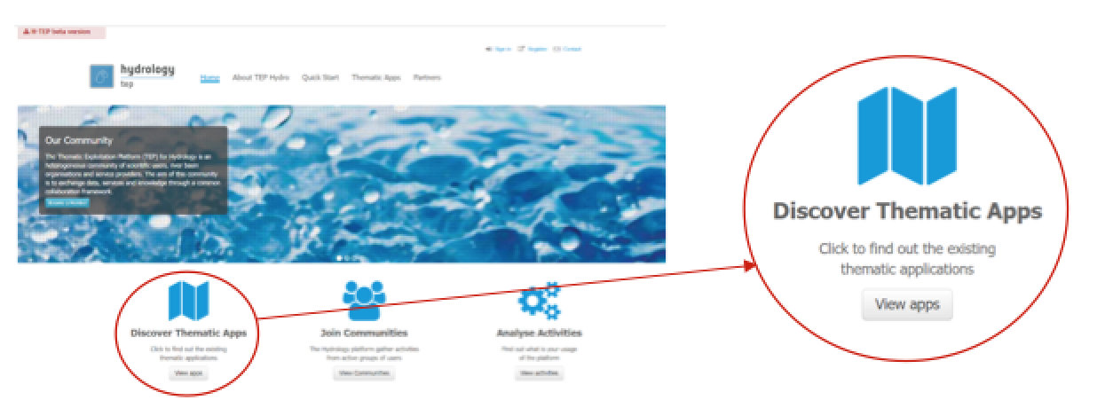
Figure 5: Step 2 - Access the thematic applications
- A list of available Thematic Applications is shown. For this tutorial the Water Quality App for Red River is used. The application can be opened by clicking on the Open App button on the right side. A pop-up containing information about this specific application and a list of some application-keywords appears when clicking on the title of the app. The Water Quality application can also be accessed directly using the URL https://hydrology-tep.eu/geobrowser/?id=waterquality-redriver.
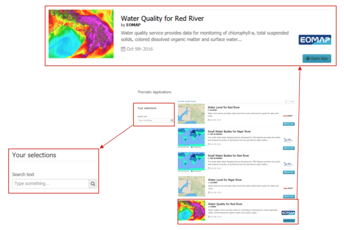
Figure 6: Step 3 and 4 - Available applications and your selections
- Filter your application of interest by using the Your selections column on the left side of the Thematic Applications page: Search text allows you to use keywords to find a corresponding thematic application. Currently the Your selections-feature is unnecessary, as there is only a limited number of thematic applications available. However, you might need this feature to find your application of interest once the number of available applications has significantly increased.
2.5.2.2. Search Your Data of Interest for Your Area of Interest
Once the Water Quality application has been accessed, a new tab opens called the Geobrowser. This part of the tutorial will teach you to work with the various features and functions available within the Geobrowser. Currently the default map is of Northern Vietnam and Southern China: the Red River basin. The default map shown upon opening the WQ app may change in the future.
- You can zoom in and zoom out by clicking on the + and – icons on the left side of the Geobrowser, encircled in red. The map can be shifted to any desired area by clicking on the map and dragging your mouse. For this tutorial the focus is kept on default; the Red River area in Northern Vietnam and Southern China.

Figure 7: Step 1,2 and 3 - The water quality application Geobrowser
- If you are correctly logged onto the HTEP platform, on the top-right of the Geobrowser your username should be displayed (2a). If you need any further explanation about the HTEP-platform and its features, a Help Guide can be easily accessed through clicking on the book-icon next to the email-icon (2b). If this is insufficient, you can ask for help through the contact form (2c). If you would like to sign out, this can also be done within the Geobrowser by the exit-icon (2d).
- You can select which satellite data source you would like to use for your research on the top-right of the Geobrowser. Selecting EO Data imposes a dropdown menu showing all available remotely sensed EO data sources for this application.
As discussed in Section 2.5.1.1.1, the WQ application has currently data available from Landsat-8 and Sentinel-2. The EO data to be selected depends on your requirements and research purposes, as each satellite has its own specifications suiting different requirements. Landsat-8 and Sentinel-2 have relatively similar specifications. They both have for example a rather high spatial resolution of 30m, meaning they are well suited for monitoring of water quality in rivers and small lakes.
For this tutorial, Landsat-8 data is selected.
- Once EO data from a certain satellite is selected, you can search for specific data images (data products) within the available database from the selected satellite. The options to filter your data products of interest out of the complete database are listed below. The actions can also be combined for an even more specific data search.
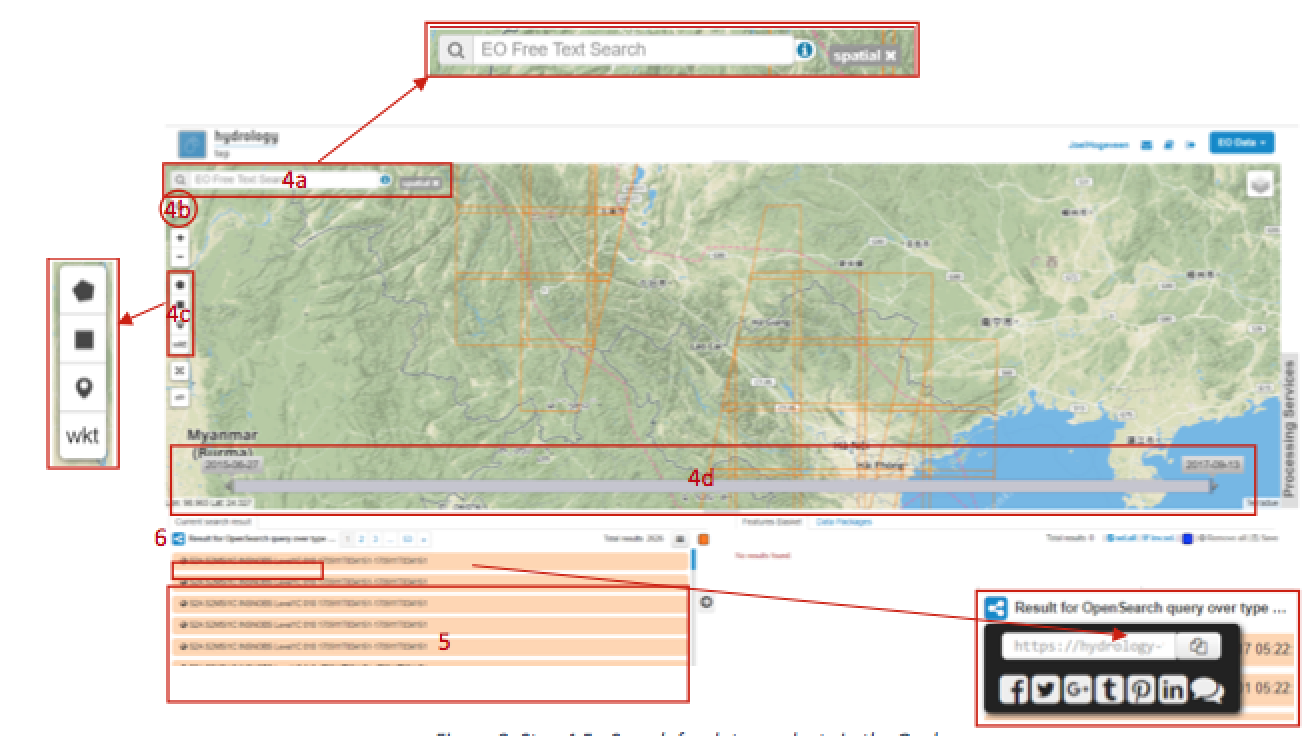
Figure 8: Step 4,5 - Search for data products in the geobrowser
➢ Search Field (4a): On the top-left of the Geobrowser, you see a search field. In this field, you can do a text search for specific EO data products within the data source chosen in step 3. For now this field is left blank.
➢ Clicking on the magnifying glass (4b) below the search field, opens the Search Panel of Figure 9: a panel containing multiple additional filters to find your desired data product. For example the productType and a time range filter. Show Other Parameters opens another extensive list of filters, amongst others cloud- and land cover filters and geometry filters for a spatial search. For now also leave the Search Panel untouched, so at default settings.
Note
The Search Field cannot be used to search for geographic places: this feature in non-existent in the Geobrowser.
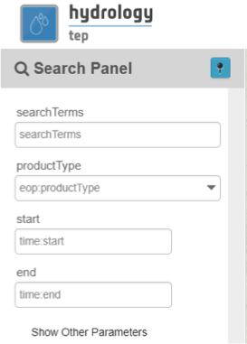
Figure 9: Data products search panel
➢ Although the Search Panel already provides you the option for a spatial filter based search, you can also apply a spatial search through the tools of 4c. A polygon, rectangle, marker and well-known text (WKT) code can be used to define your area of interest. For this tutorial a spatial filter is applied using a WKT-code. Click on the WKT button: the pop-up of Figure 10 appears.
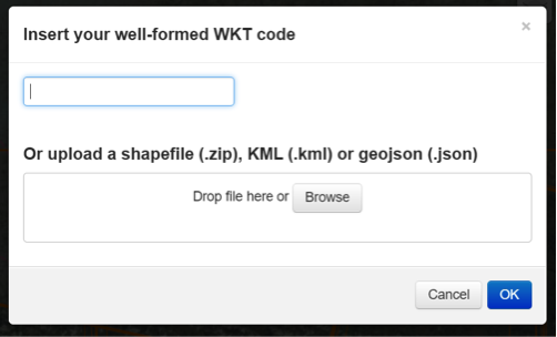
Figure 10: Step 4c - Apply a spatial filter using WKT-code or Shapefile
As you can see a spatial filter can be applied using a WKT-code, but also by simply dragging and dropping a Shapefile or uploading a Shapefile from your computer. For now a WKT-text is used. Copy and paste the following code in the top field: POLYGON((104.86 22.1,105.006 21.951,105.072 21.731,105.057 21.678,104.951 21.714,104.826 21.87,104.709 22.045,104.86 22.1)) and click on OK. This WKT code is the Yen Binh water reservoir: the reservoir should now be boxed by a pink dashed line.
➢ Now also a time filter is applied. The time filter can be applied not only through the Search Panel, but also using the tool of 4d indicated in Figure 8. The slider at the bottom is a time filter that can set by sliding the begin and end date to the desired time range. For now drag the left side of the time filter to 2017-01-01 and leave the right side of the time filter at default: 2017-05-01.
- The current search results, based on the selected satellite and the applied filters, are displayed on the bottom left of the Geobrowser. The data products in this box are also displayed on the map of the Geobrowser by means of orange rectangles. There should be 7 data products found for the search of this tutorial.
- If you would like to share your search results, click on the blue icon above the search results. The link can be copied and pasted or be posted through social media (i.e. Facebook and Twitter). Feel free to share if you like.
2.5.2.3. Select Your Data of Interest for Your Area of Interest
Figure 11 shows the search results from Section 2.5.2.2. Now the data products of interested will be selected and saved in a Data Package.
- By clicking on an EO data product in the current search results box, the selected product is highlighted blue. In the map the spatial area covered by the selected product is boxed by a bold white line and a pop-up appears. In the pop-up information about this specific data product is provided.
- In the pop-up box there is also the option to select Download or Related Search. The download can be performed through the Granule Download URL (for Landsat-8 this is through the USGS database) or directly through the Data Gateway or the HTEP platform. The related search offers you the option to search for data products with a similar time range, spatial coverage or a combination thereof as the currently selected data product. Feel free to download or do another search, but for this tutorial it is not necessary.
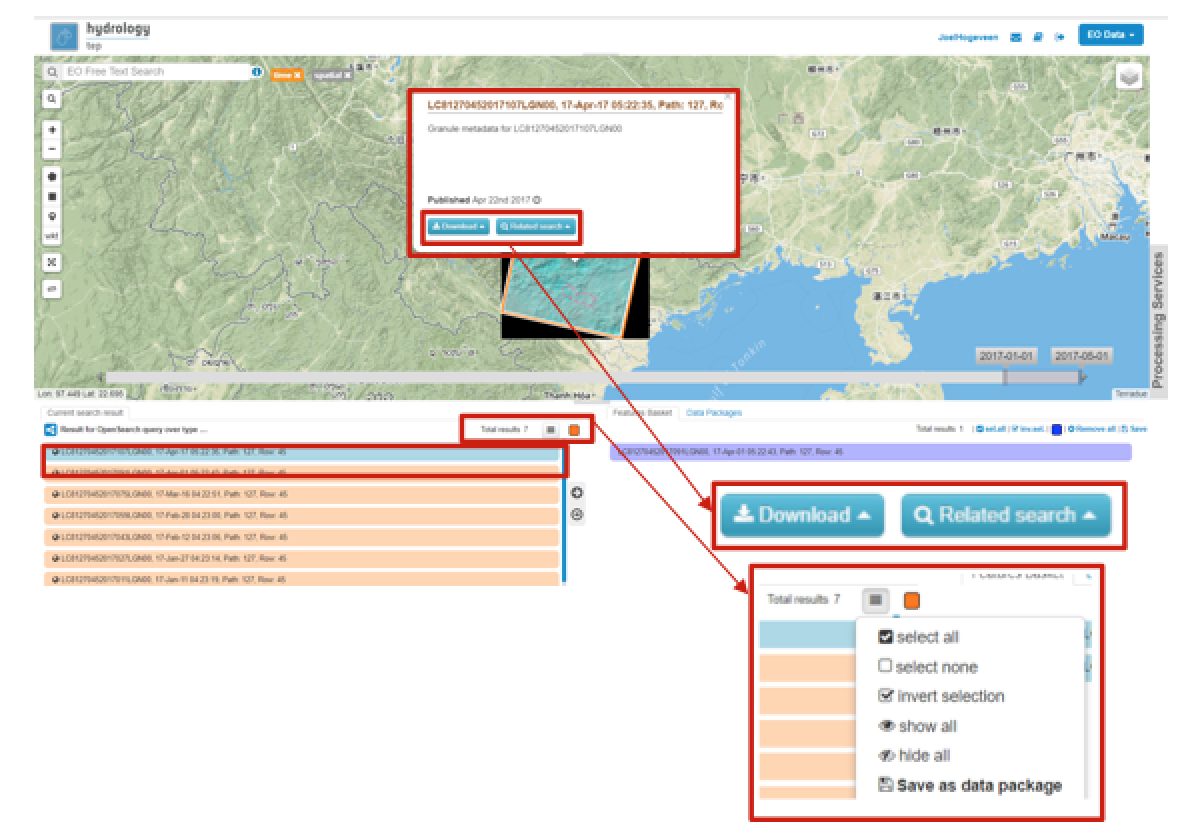
Figure 11: Step 1-4 - Select your data product of interest
- Hovering the data products in the search results will show the corresponding Landsat-8 image in the Geobrowser. As such it can be easily determined what image suits your interest.
- To easily select/deselect (multiple) products or show/hide (multiple) products on the map of the Geobrowser, use the icon next to the orange square.
- The data products of interest for your research can be selected and transferred to the features basket simply using drag and drop as illustrated in Figure 12.
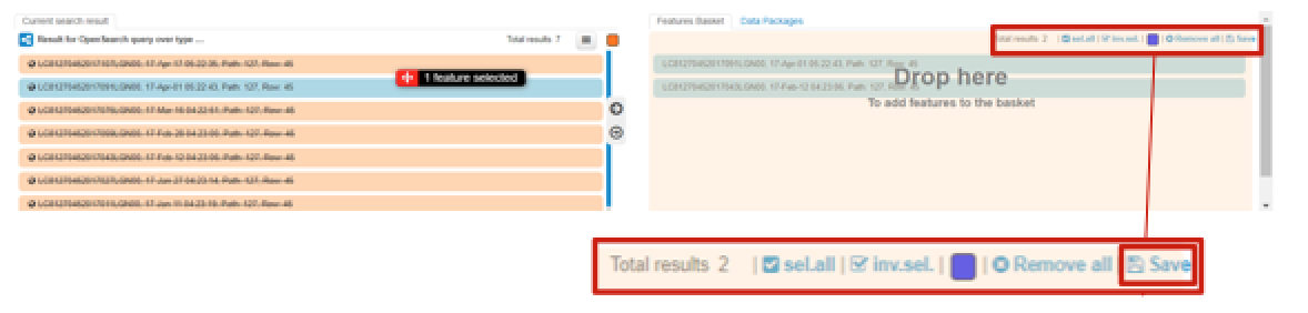
Figure 12: Step 5-7 - Drag and drop data products from search results to features basket
For the purpose of this tutorial, two data products are selected and transferred to the features basket: LC81270452017091LGN00 (cloud free scene) and LC81270452017043LGN00 (clouded scene).
- The products in the features basket can be easily selected/deselected and/or removed using the options on the top-right of the features basket.
- All data products dropped in the features basket, can together be saved as a single Data Package using the Save button on the top-right of the features basket box. The pop-up of Figure 13 appears and a name can be assigned to the Data Package. Name your data package WQ_YenBinh_Reservoir_LS8_username (replace username by your username). Click on Save to Save the Data Package: a message should appear stating a successful save.
The advantage of a Data Package is that you can easily load your data products of interest at any arbitrary time and you can also easily share it with other hydrologists.
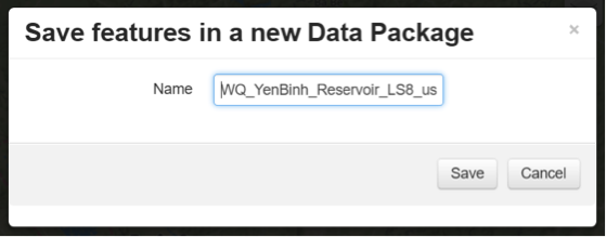
Figure 13: Step 7 - Save your data products in a Data Package
- Your data package created in step 7, can be found in the Data Packages box. Access the Data Packages box using the Data Packages tab, located next to the Features Basket tab.
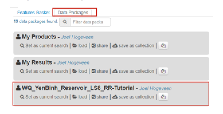
Figure 14: Step 8-10 - Overview of available data packages
- You see a list of many Data Packages published by other users. Find your own Data Package, which has the name you gave it in Step 7. The human-icon in front of the Data Package name indicates this Data Package is created by you and only visible for you.
- One of the options is to share your Data Package with all other HTEP users or with your community. To do so, click on share. A pop-up will appear as shown in Figure 15.
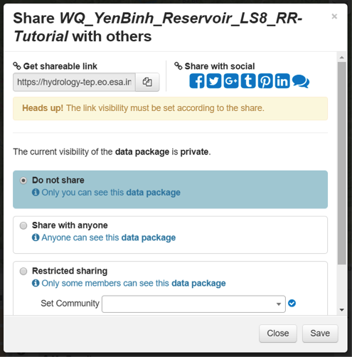
Figure 15: Step 10 - Choose the visibility of your data package
· Do not share: Default setting, meaning your data package is only visible for yourself. · Share with anyone: Share your data package with all other HTEP users. · Restricted sharing: Share your data package with a limited number of users, for example only a specific user(s) or with users from the same community. For now, leave your data package at default settings (Do not share) and Close the pop-up. In the list of public Data Packages there should be a Data Package called WQ_YenBinh_Reservoir_LS8_RR-Tutorial. This Data Package was created and published for the purpose of this tutorial. Please click on load: the same search results and data products as your own results and products so far should be loaded in the current search result box and the features basket. 11. Additional features to manage Geobrowser map visualisation: On the top-right of the Geobrowser the lay-out manager-icon, indicated by the red rectangle in Figure 16, can be selected: a list of options will appear to manage the Geobrowser map visualisation. The background of the map can be changed from default to for example Google Maps or Natural Earth. In the dropdown menu it can also be defined which products should be shown on the map: for instance the products from the related search, the products from the features basket or the data results after processing, which will be discussed in Section 2.4. Feel free to play with the visualisation of the map.
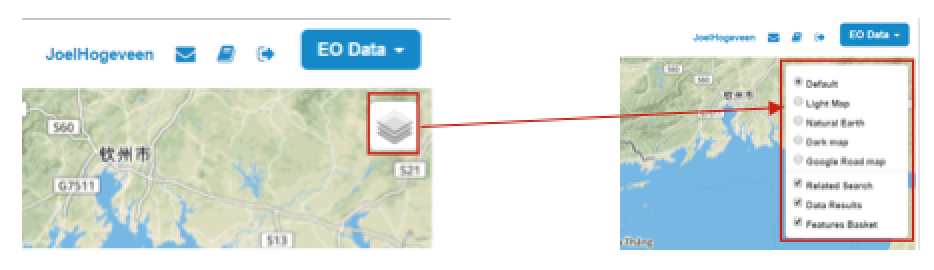
Figure 16: Step 11 - Change the visualisation of the Geobrowser map
2.5.2.4. Processing Your Data Using the Water Quality Service
Section 2.5.2.2 and 2.5.2.3 explained how to search for and select your data of interest within the Geobrowser. Having the relevant data selected and saved, it is now time to process this data to obtain the desired product output.
- The processing services can be accessed from within the Geobrowser, but they are initially hidden. Open the available processing services by clicking on the processing services tab.
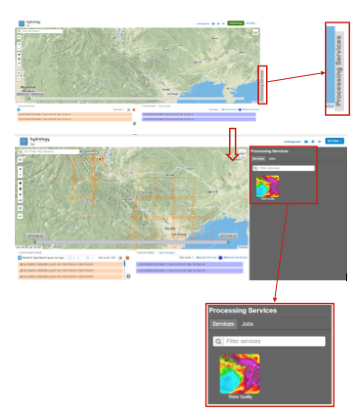
Figure 17: Step 1, 2 and 3 - Access processing services
- On top of the processing services, three options are displayed: Services, Jobs and a Search Field.
➢ Services: This tab yields a list of available processing services (the different models and algorithms within the application). Currently only the Water Quality processing service is available, but this number will increase in the future.
➢ Search Field: Once the number of available processing services has increased, the Search Field can be used to filter only those processing services of interest.
➢ Jobs: This tab lists all existing jobs. The jobs shown are the jobs you have created yourself or the jobs who have been published by other HTEP users.
- For now, click on the process service Water Quality to access the Water Quality processing service. See Figure 18.
- To process data and create output, a Job needs to be created. A job can be created by filling in all the fields as shown in Figure 18:
➢ Job title: Give your Job a title, for instance WQ_YenBinh_Reservoir_LS8_Spring2017. Any other name with arbitrary length and symbols is also allowed.
➢ Select Input Files: Here you define which products should be analysed. To provide the processing service with your to-be-analysed products of interest, simply drag and drop your product from the features basket (or straight from the search results) to the field. Multiple products for analysis can be selected by clicking on the -icon next to the field.
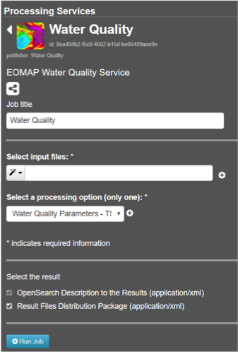
Figure 18: Step 3,5 - Water quality processing service
As an alternative, you can also click on the arrow on the left of the field: a menu will drop down, where one can choose between current bbox (bounding box) from geometry, current geometry or current bounding box. The products that cover the area of your pick (this area is based on the defined spatial filter applied in Step 4 of Section 2.1), are then automatically selected.
For now the two products in your features basket will be selected for analysis by dragging them from the features basket to the Select input files fields in the processing service. If desired, you can share your processing service on social media with the Share-icon above Job Title.
➢ The last step is to Select (output) Products: The default output product are all available Water Quality Parameters. If you click on this field, a dropdown menu appears providing you the option to also analyse the Atmospheric Corrected image or even both.
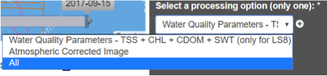
Figure 19: Step 4 - Available output products
➢ For now All is selected.
- Lastly you need to select the result. By default Result Files Distribution Package is selected, which means that the results will be shown within the Geobrowser (and in xml-format) after the job-analysis is finished. Therefore this option is kept as default.
- Click on Run Job to run the job.
- Now the job is running, your data is analysed using HTEPs cloud services. During the processing of your data, information about your job is displayed as shown in Figure 20. Job Info provides info about the job, such as the name of the job, its identifiers, the date of creation and the user who created the job. Besides a progress bar shows you the progress of the analysis and under parameters you see the input and output parameters used for this specific job.
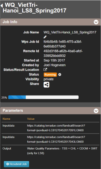
Figure 20: Step 7 - Job progress and job info
2.5.2.5. Visualising and Sharing of Job Results
The previous section showed how to process the data products obtained from Section 2.5.2.2 and 2.5.2.3. Once the process is finished, which may take a considerable amount of time, the results can be visualized and possibly shared with others users and/or your community.
- Once the processor has finished the job, the Status of the job will change from Running to Success as shown in Figure 21.
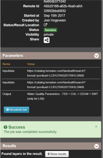
Figure 21: Step 1-3 - Processor after sucessful job
- If a problem occurred during the processing of your job, or if it was performed using the wrong parameters then click Resubmit Job to run the job again. Adaptions to your parameters can be made.
- But if your job was processed correct and successful, simply click on the Show Results button to show the results of your job.
- The results of your job are loaded in what previously was the current search result box, see Figure 22. To know if you this box contains EO satellite data products or job results, take a look on the top-right of the Geobrowser to check if you are in the Products tab or EO Data tab.
- The job results are not just loaded in the current search results box, but also in the Geobrowser. You can visualize each parameter individually in the Geobrowser by selecting the option show only this feature.
- Each product shows the results for a specific parameter. Furthermore the included QUC and QUT files can be used for quality control and an overview of the reliability of the results. Please have a look at Chapter 5.4.3. of the User Manual for an elaborative description on how to interpret the product results: http://hydrology-tep.github.io/documentation/apps/wq.html. Notice the obvious differences in results and quality between the processed data product covered by clouds, and the cloud free data product.
- The resolution of the job results within the Geobrowser is rather low and may impose the false assumption of unreliable results. Therefore, click on your data product of interest in the result box and a pop-up will appear as shown in Figure 22. Here you can Download the result in different formats.
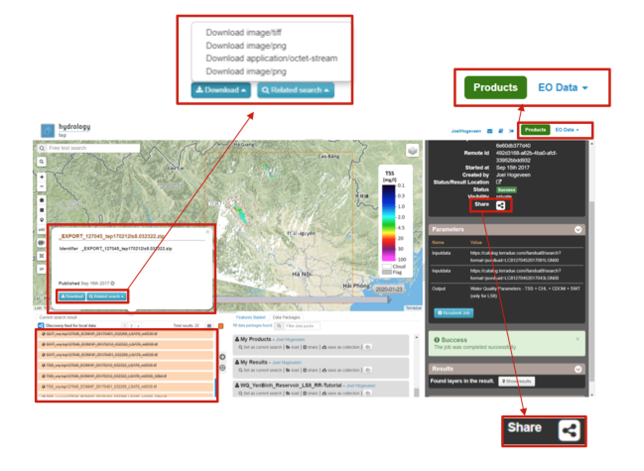
Figure 22: Step 4-8 - Visualisation of Job Results
- Trough the Share-button in the processor tab, you can share your results with other users, your community, or simply with all HTEP users.
- To find your previously generated job results, or to find job results shared by others users, go to the Jobs-tab in the processing service as illustrated in Figure 23.
- Click on the Show thematic jobs-field next to the Filter Jobs Search Field: here you can choose which jobs you wish to see: thematic jobs, all jobs, on your own created jobs or only public jobs. Once you found your job of interest, simply click on the name of your job and access the results as explained in steps 3-7. There is a thematic job available that shows the results from this tutorial: WQ_YenBinh_Reservoir_LS8_Spring2017.

Figure 23: Step 10 - List of published Jobs