6.3. Hydrological Modelling
The aim of the Hydrological Modelling Application is to provide a platform for assimilation of EO data in hydrological models. It includes processing services for running a hydrological model in hindcast and forecast mode with or without satellite and in-situ data assimilation, accessing meteorological data from external data services, preparing EO data for assimilation in the hydrological models, basic visualization and statistical analysis of model results.
The Hydrological Modelling Application is implemented using the Niger-HYPE model (v2.21) providing simulations of river discharge, lake water level and outflow, as well as land surface water balance components (precipitation, evapotranspiration, runoff, and soil water content) for the Niger river basin. The service collects meteorological forcing data from the SMHI Global Forcing Data service for simulations of historical periods from 1979 until current time, and short to medium range forecasts (1-10 days) since 2016-06-01. The following four Processing services are included in the application:
- Niger-Hype simulation of historical period
- Niger-HYPE forecast
- EO-data pre-processing
- Return Period magnitude Analysis
Further details about the Niger-HYPE model http://hypeweb.smhi.se/niger-hype Source code and information about the HYPE model see http://hypecode.smhi.se Documentation and wiki about HYPE that can be useful in the following hands-on exercises is found here http://www.smhi.net/hype/wiki/doku.php
6.3.1. Access to the thematic application
The Hydrological Modelling application is accessed from the home page of the Hydrology TEP community portal:
- Enter the HEP portal and sign in with your HEP community user account https://hydrology-tep.eu
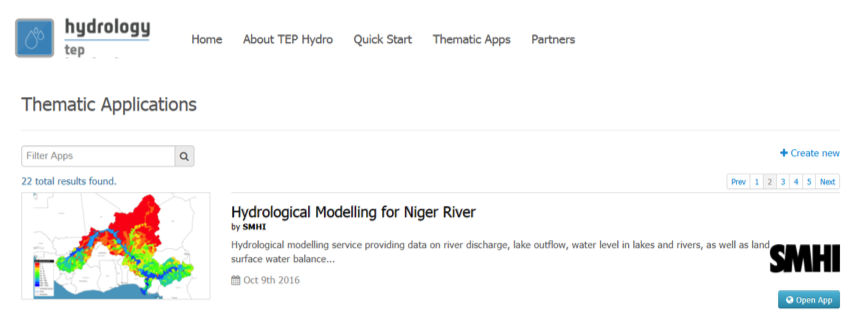
- Open the list of Thematic applications with the view_apps link below the Discover Thematic Apps icon.
- Find the link to the Hydrological_modelling application (Open App):
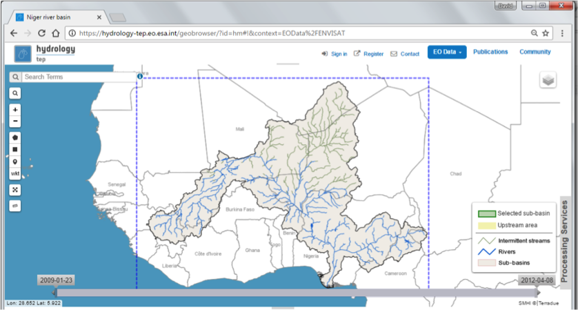
- The initial view of the hydrological modelling application showing the Niger-River drainage basin in the Geobrowser as represented in the Niger-HYPE [1] model.
| [1] | See http://hypecode.smhi.se and http://hypeweb.smhi.se/nigerhype for more details about the hydrological model HYPE and the Niger-River HYPE model application, respectively. |
- Selection of area of interest based on drainage basins and upstream area:
- Integrated in the Geobrowser is a functionality to select area of interest for EO data exploitation based on the hydrological model sub-basins and their upstream area
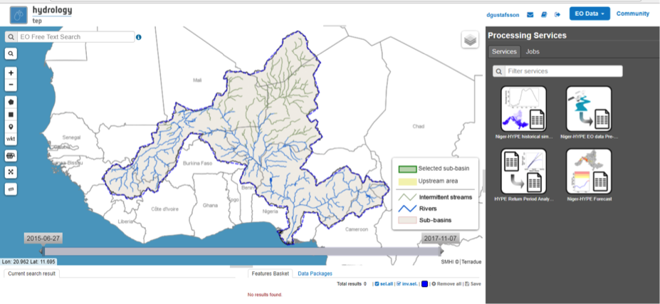
- Hydrological Modelling Processing Services are found on the Processing Services tab on the right side of the geobrowser:
- Niger-Hype simulation of historical period
- Niger-HYPE forecast
- EO-data pre-processing
- Return Period magnitude Analysis
Instructions how to run the different processing services are given in the following sections.
6.3.2. Selecting the Area of Interest based on drainage basins and upstream area
The hydrological model sub-basin layer makes it possible to select area of interest based on drainage basins and upstream area.
This functionality is dependent on the drainage basin data set available on the portal.
Currently, the drainage basin of the Niger river as represented in the Niger-HYPE model is the only dataset loaded into the HEP community portal.
6.3.2.1. Select a sub-basin and it’s upstream area in the Geobrowser
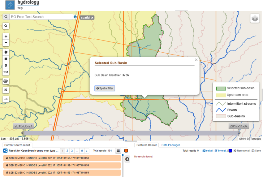
- Zoom in to the area of interest and select a sub-basin by clicking in the map (left mouse button) [2] . The selected sub-basin is highlighted in green, and the upstream areas in yellow.
- To select another sub-basin, click in another non-highlighted basin (it’s not possible to select a sub-basin from the current selected upstream area)
| [2] | The EO data coverage polygons may be blocking the sub-basin polygons. Solution, see Known issues. |
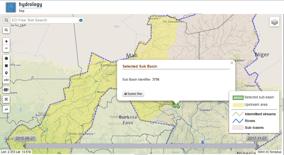
- Click a second time in the selected sub-basin and a pop-up dialogue will appear with information about the sub-basins identifier in the Niger-HYPE model.
There is also functionality for applying spatial filter on the EO data selection, see further below.
- Known issues
- It is not possible to select sub-basins that are covered by an EO data coverage polygon. Try to reduce the EO data selection by changing data set or by using the time filter.
- To select a sub-basin in the current selected upstream area, the selected region must first be de-selected, which can done by selecting a non-highlighted sub-basin in another part of the model domain.
6.3.2.2. Spatial filtering of EO data using the hydrological model sub-basins
- Select the sub-basin of interest by mouse click in the geobrowser.
- Select the EO data of interest from the EO data drop-down menu at the top-right of the portal.
- Click a second time in the sub-basin of interest, and apply the spatial filter in the pop-up dialogue.
The method will select the EO data that are covering the selected sub-basin only.
By clicking somewhere in the upstream area, the spatial filter will be applied using the upstream area.
The selected data sets can be added to the Feature basket and used for processing within the other thematic applications.
6.3.3. Run the Niger-HYPE historical simulation Processing Service
This hands-on exercise describes how to make simulation with the Niger-HYPE historical period service with or without EO data assimilation.
6.3.3.1. Running the Niger-HYPE historical simulation processing service
- Open the Niger-HYPE historical simulation service and Select name for you job in the Job title parameter field
- (mandatory) Set the start of the simulation period in the Start of simulation (yyyy-mm-dd)* input parameter field (obligatory).
- In the example 2016-04-01 (the start of the rainy season in the Niger river basin is usually in the beginning of April)
- (mandatory) Set the end of simulation period in the End of simulation (yyyy-mm-dd)* input parameter field:
- In the example 2017-03-01 to produce a one-year simulation.
- (mandatory) Select outputs from the fixed list of available simulated variables in the Output variables drop down menu:
- The output variable list is build up of three components on the format Variable Name (unit) [4-letter code used internally in the HYPE model]
- Click the + sign to enable selection of more variables.
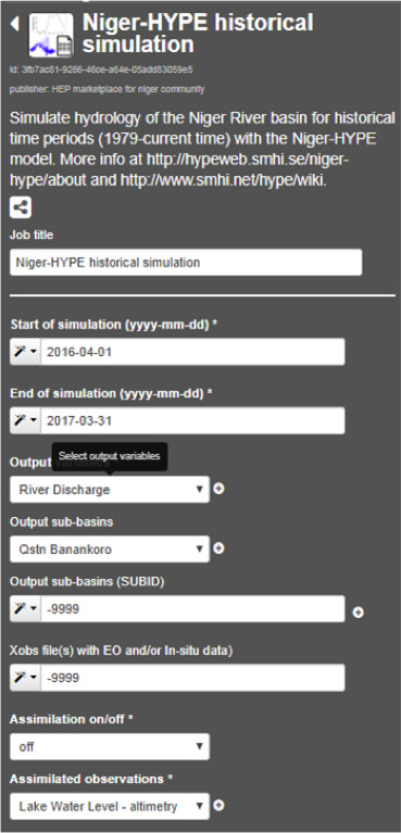
- (mandatory) Select output locations (sub-basins in the Niger-HYPE model) from a fixed list of named locations in the Output sub-basins drop down menu:
- The output location list includes all sub-basins in the Niger-HYPE model where there is a discharge station (Qstn) or a outlet lake (Lake). The name of the discharge station/lake and the sub-basin identifier are included in the drop down list.
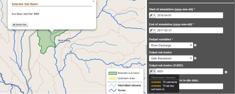
- (optional) Select additional output locations that are not listed in the Output sub-basins list by entering the sub-basin identifier in the Output sub-basins (SUBID) input field:
- The sub-basin identifier can be found for any basin in the model by clicking on the basin in the map browser. It is also possible to set the sub-basin identifier in the input field by using the magic tool in the left side of the input field and select “subbasin id”
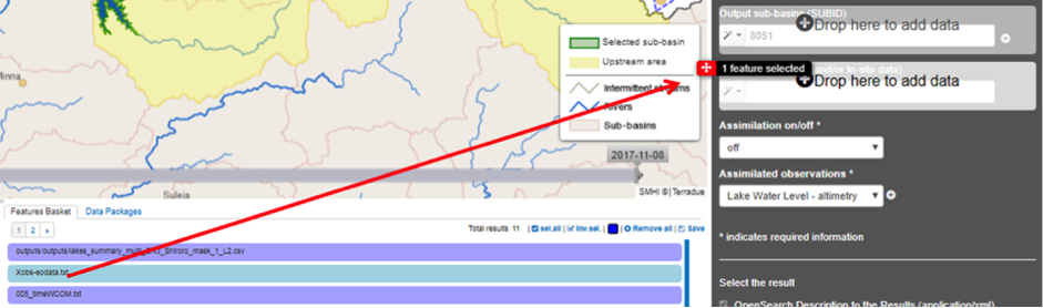
- (optional) Add and so-called Xobs-file with pre-processed EO or in-situ data to the model simulation by dragging an available data set from your Features basket:
- An example can be found in a public data package called Niger-HYPE RPM check data set, which includes a data set called Xobs-eodata.txt with a time-series of lake water level from Lake Shiroro generated with the Water Level application.
- (optional) Switch Data Assimilation on or off in the Assimilation on/off input field:
- Switching assimilation on will trigger an Ensemble Kalman filter assimilation run, where the data inserted in the previous step is used to adjust the model simulation towards the assimilated data.
- (mandatory of Assimilation is On, otherwise optional) Select which variables to be assimilated in the Assimilated observations input field. Currently it is only possible to select one of two options:
- Lake Water Level Altimetry AOWL WCOM (altimetry based lake water levelis assimilated if a variable called AOWL is present in the Xobs-files entered in the previous input field)
- Openloop ensemble simulation without assimilation OPEN LOOP (the same type of ensemble simulation is generated as for an assimilation run, however no observations are assimilated).
Please note that the ensemble simulations generated when switching Assimilation On requires much more processing time (at least 10 times more) compared to Assimilation Off. This is due to two reasons:
- The Ensemble Kalman filter method is based on ensemble simulations. Currently, the Niger-HYPE application is configured to include 10 members in the model ensemble (which is actually already a rather small number, 50 or more would be better).
- The model ensemble must also have enough variability to be able to adjust to the observations in a realistic way. Currently, the only method used here to generate ensemble spread is to add random perturbations to the meteorological forcing data (precipitation and temperature). Thus, it becomes important to include at least one rainy season in a warm-up period before the assimilation period. Consequently, the selected start of the simulation period is automatically adjusted to meet this criteria.
It is advisable to first make a simulation without assimilation to check results, and also the bias between simulated variable (WCOM in the example) and the observations to assimilate (AOWL in the example) and possibly correct the offset input parameter in the EO data pre-processing (see section 6.3.5 below).
6.3.3.2. Results from the Niger-HYPE historical simulation service
The results from the processing service is described in the table below. The prefix numbers are used as a trick to order the output files in a certain order.
| Output files | Description |
|---|---|
| 001_[subid]_[name].png 001_[subid]_[name].pngw | Quicklooks (PNG format with associated word file PNGW for visualization in the map browser) with time-series plots of simulated variable [name] for sub-basin [subid], where [name] corresponds to the 4-letter code for HYPE model variables and [subid] to the Niger-HYPE sub-basin identifier. |
| 001_map[name].png 001_map[name].pngw | Quicklook (PNG format) with maps of variable [name] with mean simulated variable during the simulation period, where [name] corresponds to the 4-letter code for HYPE model variables. |
| 002_[subid].csv 003_[subid].txt |
Each text file includes data for the entire simulation period (daily values) for all selected output variables for one sub-basin. |
| 004_map[NAME].txt | Text file with average (full simulation period) simulated value for a selected variable specified by the file name (4-letter variable names, see HYPE wiki pages). Each row represents one subbasin of the model. |
| 005_time[NAME].txt | Text file with average (full simulation period) simulated value for a selected variable specified by the file name (4-letter variable names, see HYPE wiki pages). Each row represents one subbasin of the model. |
| 006_simass.txt 006_subass.txt | Text file with assessment of the agreement between simulated and observed data (depending on which observed variables added to the simulation through the Xobs-files). |
| 009_hyss_000_YYMMDD_hhmm .log | Log-file for the HYPE model simulation |
| hypeapps-historical- logfile.txt | Log-file from the processing service. |
6.3.4. Run the Niger-HYPE Forecast Processing Service
This hands-on exercise describes how to make a forecast simulation with the Niger-HYPE historical period service with or without EO data assimilation. Please note that several steps are identical to the Niger-HYPE historical simulation service. In this case, the hands-on guide will refer to section 6.3.3
The forecast service always makes two simulations - first a 3-month warm-up simulation (the hindcast) ending on the day before the start of the 10-day forecast simulation (the forecast). The outputs from hindcast and forecast simulations are published separately in the application results. The first day of the forecast simulation is called the Forecast issue date, and is one of the input parameters to the applications. Data is saved in the system to enable forecasts for issue dates between 2016-06-01 until the day before the current date.The application may automatically adjust the forecast issue date to an earlier date if the update of the meteorological forcing data for some reason is lagging behind (update is usually made around noon every day).
6.3.4.1. Running the Niger-HYPE forecast processing service
- Open the Niger-HYPE forecast service and select Job Title (same procedure as in 6.3.3)
- (mandatory) Set the start of the 10 day forecast simulation in the Forecast issue date (yyyy-mm-dd) input field.
- (mandatory) Select output variables and output locations (same procedure as in 6.3.3)
- (optional) Enter a custom made Return Period Warning Level File for the calculation of river discharge forecast warning levels (or leave “default” to use the default data embedded in the aplpication, representing 2,5, and 30 years return period for warning levels 1, 2, and 3, respectively, based on a historical simulation 1979-2013).
- (optional) Set parameters for Xobs inputs and Data assimilation (same procedure as for 6.3.3)

6.3.4.2. Results from the Niger-HYPE forecast processing service
First of all, the Niger-HYPE forecast service produces similar results as the Niger-HYPE historical service - all variables listed in the section 6.3.3.2 are produced both for the hindcast and the forecast simulation period, except for the quicklooks. Results are sorted in subfolders called forecast and hindcast, respectively.
In addition, three specific forecast outputs are generated by the forecast service, and at the end also a processing service log file:
| Output files | Description |
|---|---|
| 001_[subid]_discharge-forecast.png 001_[subid]_discharge-forecast.pngw | River discharge forecast time-series plots (png quicklooks) for the selected output sub-basins [subid], with the return-period levels based warning levels plotted in the background. The quicklooks are visualized in the map browser located with the lower left corner in the centre-coordinate of the corresponding basin. |
| 001_mapWarningLevel.png 001_mapWarningLevel.pngw | River discharge forecast warning level maps (png quicklooks), showing the maximum forecasted river discharge warning level in each sub-basin of the Niger-HYPE model. The quicklook is displayed in the map browser scaled to the current map scale and centered on the Niger River basin. |
| 004_mapWarningLevel.txt | Maximum forecasted river discharge warning level in the HYPE map output text format (same format as 004_map[NAME].txt) |
| hypeapps-forecast-logfile.txt | Log-file from the processing service. |
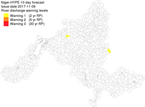

Example of River discharge forecast warning level map output (left) and River discharge forecast time-series output (right).
6.3.5. Run the EO Data Pre-processing Processing Service
The purpose of the service is to transform data sets generated by the H-TEP EO data services to the time-series format required by the hydrological model. This include both spatial and temporal aggregation of the EO data sets. Currently, the service is configured to do temporal aggregation of data from the Water Level service, to provide time series with data representative for a selected Niger-HYPE sub-basin. The output is a textfile in the specific Xobs text format required to be assimilated in the HYPE model (see further on the HYPE wiki pages).
6.3.5.1. Running the Niger-HYPE EO data pre-processing service
This section provides a brief guideline on how to use the Niger-HYPE EO data pre-processing processing service to prepare data from the Water Level service for assimilation in the Niger-HYPE model:
- (mandatory) Make sure you have available in your Feature basket a relevant data set with water level time-series data generated by the H-TEP Water Level service.
- An example is available in the public data package called Niger-HYPE RPM check data set, which includes a data set called lakes_summary_multi_SN3_Shiroro_mask_1_L2.csv, with a time-series of lake water level from Lake Shiroro (subid 212) generated with the Water Level application.
- This data package also contains the expected output of this exercise called Xobs-eodata.txt, which can be used to check the output.
- Enter the EO data pre-processing service, and edit the job name in the Job Title input field.
- (mandatory) Drag the Water level data set from Feature basket into the Water Level Time-series Data, EO or In-situ (*.csv) input field.
- Use the lakes_summary_multi_SN3_Shiroro_mask_1_L2.csv from the example or your own data set.
- (mandatory) Set the sub-basin identifier corresponding to the EO data set in the Sub-basin identifier - one for each dataset input field
- Lake Shiroro corresponds to Niger-HYPE sub-basin 212.
- (mandatory) Select the HYPE model variable corresponding to the EO data in the HYPE variables - one for each dataset input field:
- Lake water level altimetry (m) AOWL for altimetry data, or
- Lake water level in-situ (m) WSTR for in-situ data
- (mandatory) Set the vertical Offset correction of the EO (or in-situ) data set:
- This parameter is useful for reducing the mean bias between the model and the observations - which is important if the data is intended for assimilation in the model. The data assimilation method can only adjust the bias to a certain extent, and is more efficient to adjust temporal errors if the mean bias is small.
- The offset is an additive correction of the EO data, and can be a negative (EO data is corrected downwards) or positive number (EO data is corrected upwards).
- It is recommended to make an initial comparison with the simulated lake water level using offset=0, and then redo the pre-processing with a correction factor estimated from this initial comparison before assimilating the EO data in the model.
6.3.5.2. Results from the Niger-HYPE EO data pre-processing service
The results from the EO data pre-processing service is a text file called Xobs-eodata.txt containing the analysed EO data in the HYPE models Xobs-format:
- one row for each date (please note how the dates with missing data is padded with missing value identifier -9999)
- and one column for each variable and sub-basin (please note the format of the two header rows containing the sub-basin identifier and the 4-letter coded HYPE model variable names, respectively).
- Move the xobs-eobs.txt from the results container to the Feature basket if you intend to use it for assimilation in the Niger-HYPE modelling processors (historical or forecast).
In addition, there is a processor log file generated, which indicate if some input caused unexpected behaviour of the processor.
6.3.6. Run the Return Period Magnitude Analysis Processing service
The purpose of the HYPE Return Period Analysis processing service is to estimate annual maximum values of for instance daily mean river discharge or precipitation at selected return periods (years). These return period levels (or magnitudes) can be used as input to the Niger-HYPE forecast processing service as thresholds for forecast warning levels. Currently, the Niger-HYPE forecast service will only use return level estimates for river discharge, but the HYPE Return period Analysis service can be used to analyse any output variable from the HYPE model (given in the time output format, which is generated by the Niger-HYPE historical processing service.
6.3.6.1. Running the HYPE Return Period Analysis processing service
This section provide a brief guide on how to make use of the return period analysis service.
- (mandatory) Make sure you have time-series outputs from the Niger-HYPE historical simulations processing service available in the Feature basket:
- It should be a dataset in the HYPE time-output format, time[NAME].txt
- It should cover as long time-period as possible (if possible, close to the maximum return period you would like to estimate level for)
- Examples are available in the public data package Niger-HYPE RPM check data set, for instance the river discharge dataset 005_timeCOUT.txt
- Open the HYPE Return Period Analysis service and edit the Job Title if needed.
- (mandatory) Drag the selected time-output data from the Feature basket into the HYPE timeoutput data (time****.txt) input field.
- (mandatory) Set the requested return periods for the analysis in the Return Periods (years) input field (for instance 2,5,30).
- Run the application
6.3.6.2. Results from the HYPE Return Period Analysis processing service
The result of the HYPE Return Period Analysis processing service is a textfile with estimated levels (annual maximum values of the input data) at different return periods (years):
- Each row correspond to a sub-basin in the Niger-HYPE model, identified by the sub-basin identifier in the first column.
- The remaining columns contain the estimated levels for the return periods (years) identified from the header row.
- Copy the result to your Feature basket if the file should be used as input to the Niger-HYPE Forecast processing service.